JSON to PDF Magic: Harnessing LaTeX and JSON for Effortless Customization and Dynamic PDF Generation
In this article, we show how to control the layout and content of the PDF document via the JSON body of the API call. We present three different JSON examples and produce three different types of documents using the same end-point. In each case, making changes to the PDF is done by editing the JSON payload. To do this, we utilise the power of LaTeX to control the layout of the PDF document.
What is LaTeX?
LaTeX is a programming language specifically designed for creating PDF documents. Source files in LaTeX have a .tex extension and are usually compiled into PDF format. While it's highly popular in academia for crafting dissertations and scholarly articles, LaTeX is also excellent for producing visually appealing documents. Its strength lies in the separation of content and stylistic rules, allowing for precise control over the document's appearance. However, a significant drawback of LaTeX is the steep learning curve involved in mastering the language for document layout.
PDF Generation via JSON to PDF
In many cases, PDF generation requirements change, and developers need to perform additional development by changing the PDF template and then ensuring the new design/changes works as expected. This process can be time-consuming. We introduce a new template called General JSON to PDF Template, which lets API users change the layout and content in one source, the JSON body of the API call. By simply changing the JSON to create a different output, developers do not need to alter templates. This simplifies the PDF generation process and gives developers an edge.
Getting Started
To get started, we will use General JSON to PDF Template end-point:
The corresponding JSON payload structure for the end-point is as follows:
{
  "documentSettings": {
    "font": "roboto",
    "fontSize": 8,
    "primaryHEXColour": "343D49",
    "secondaryHEXColour": "0dbb72",
    "textHEXColour": "444444",
    "documentName": "General JSON to PDF Template from ADVICEment",
    "topMargin": "-0.1cm",
    "rightMargin": "1cm",
    "bottomMargin": "-0.1cm",
    "leftMargin": "1cm",
    "headheight": "3.13cm",
    "headsep": "0.5cm",
    "footskip": "1.5cm",
    "includehead": true,
    "includefoot": true,
    "showframe": true,
    "header": {
      "headerLine": false,
      "leftContent": "",
      "centerContent": "\\begin{tikzpicture}[remember picture,overlay] \\node at ([xshift=0.00cm, yshift=-1.5cm]current page.north) {\\bfseries\\color{black}\\Huge{HEADER}}; \\end{tikzpicture}",
      "rightContent": "",
      "adjustMargin": "1cm"
    },
    "footer": {
      "footerLine": false,
      "leftContent": "",
      "centerContent": "\\begin{tikzpicture}[remember picture,overlay] \\node at ([xshift=0.00cm, yshift=0.75cm]current page.south) {\\bfseries\\color{black}\\Huge{FOOTER}}; \\end{tikzpicture}",
      "rightContent": "",
      "adjustMargin": "1cm"
    },
    "latexPreamble": "\\definecolor{Blue}{HTML}{00FFFF}"
  },
  "documentContent": {
    "content": [
      {
        "type": "latex",
        "content": "Some content here with LaTeX commands",
        "order": 1
      }
      ]
  }
}
This JSON object contains two main keys: "documentSettings" and "documentContent". It is a configuration file for generating a PDF document using LaTeX, a typesetting system used for creating high-quality documents. The "documentSettings" key describes various settings for the document, such as font, font size, colors, margins, header/footer details, while "documentContent" key describes the layout of the document using LaTeX commands.
"documentSettings":This key contains an object with properties related to the overall document settings."font":An optional string which contains the font of the document. Possible options are: 'helvetica', 'avant garde', 'sans serif', 'charter', 'open sans', 'bera', 'venturis', 'raleway', 'overlock', 'roboto', 'spectral', 'clear sans', 'noto sans', 'noto mono', 'josefin', 'bera sans', 'latin modern', 'theano modern', 'droid sans', 'fira sans', 'XCharter', 'bookman', 'gyre bonum', 'gyre schola', 'gyre termes'."fontSize":An optional integer which contains the font size of the document. Possible options are: 8, 9, 10, 11, 12, 14."primaryHEXColour", "secondaryHEXColour", "textHEXColour":Define the primary, secondary, and text colors using their respective HEX codes."documentName":Sets the document name to "General JSON to PDF Template from ADVICEment"."topMargin", "rightMargin", "bottomMargin", "leftMargin":Define the margins of the document."headheight", "headsep", "footskip":Define the header height, header separation, and footer skip values."includehead", "includefoot":Specify whether to include the header and footer in the document."showframe":Indicates whether to display the frame around the document."header" and "footer":Define the properties of the header and footer, such as:"headerLine" and "footerLine":Specify whether to display a line for the header and footer."leftContent", "centerContent", "rightContent":Define the content for the left, center, and right parts of the header and footer."adjustMargin":Sets the margin adjustment for the header and footer.
"latexPreamble":Contains LaTeX commands which are included before '\begin{document}' in the LaTeX file.
"documentContent":This key contains an object with a "content" property that holds an array of content elements to be included in the document."type":Specifies the content type, in this case, "latex". Possible options are: 'heading', 'section', 'subsection', 'paragraph', 'newpage', 'enumerate', 'itemize', 'kable' and 'chart'."content":Contains the LaTeX-formatted content to be included in the document."order":Specifies the order in which the content should appear.
In summary, this JSON object defines a configuration for a PDF document created using LaTeX. The document settings include font, font size, colors, margins, header/footer configurations, and a custom color defined in the LaTeX preamble. The document content is specified as an array of elements, each with a type, content, and order.
JSON to PDF with Dynamic Images
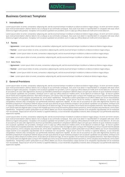
In this section, we provide an image of the PDF, which contains a dynamic image. This hands-on approach offers valuable insights into the versatility and power of using JSON to control the layout and content of your PDF documents through API calls.

The image in the JSON are generated using the \\advGetImage function. The JSON component looks as follows:
{
  "documentSettings": {
    "font": "open sans",
    "fontSize": 8,
    "primaryHEXColour": "343D49",
    "secondaryHEXColour": "0dbb72",
    "textHEXColour": "444444",
    "documentName": "Contract Template from ADVICEment",
    "topMargin": "0.5cm",
    "rightMargin": "1cm",
    "bottomMargin": "0.5cm",
    "leftMargin": "1cm",
    "headheight": "1.25cm",
    "headsep": "0.75cm",
    "footskip": "1.0cm",
    "includehead": true,
    "includefoot": true,
    "showframe": false,
    "header": {
      "headerLine": true,
      "leftContent": "",
      "centerContent": "\\advGetImage{key = logo, typeKey=logoType, widthKey = logoWidth}\\medskip",
      "rightContent": ""
    },
    "footer": {
      "footerLine": true,
      "leftContent": "",
      "centerContent": "\\thepage",
      "rightContent": ""
    }
}
....
The \\advGetImage function in the JSON file is used to insert images dynamically into the generated PDF. The function appears in the "header" section of the JSON file, indicating that it is used to display a logo in the header of the PDF document.
The \\advGetImage function has the following parameters:
key: Represents the key to access the image data (base64-encoded string) in the JSON. In this case, the key is "logo".typeKey: Represents the key to access the image type (e.g., PNG, JPEG) in the JSON. In this case, the key is "logoType".widthKey: Represents the key to access the image width in the JSON. In this case, the key is "logoWidth".
When the PDF is generated, the \\advGetImage function retrieves the image data, type, and width from the JSON file using the provided keys. Then, it embeds the image into the PDF document with the specified width, maintaining the aspect ratio of the original image.
JSON to PDF with Dynamic Tables
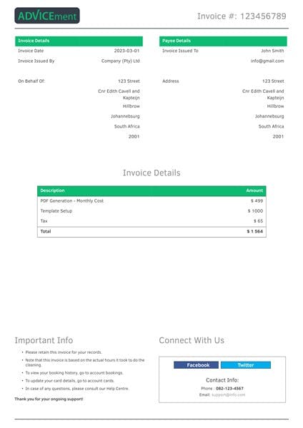
In this section, we provide both an image of the PDF and a part of the corresponding JSON body of the API call used to generate it. As shown below, this PDF contains dynamic tables, which are discussed in this section.

{
  "documentSettings": {
    "font": "clear sans",
    "fontSize": 8,
    "primaryHEXColour": "343D49",
    "secondaryHEXColour": "0dbb72",
    "textHEXColour": "444444",
    "documentName": "Invoice Template from ADVICEment",
    "topMargin": "0.5cm",
    "rightMargin": "1cm",
    "bottomMargin": "0.5cm",
    "leftMargin": "1cm",
    "headheight": "1.25cm",
    "headsep": "0.75cm",
    "footskip": "1.0cm",
    "includehead": true,
    "includefoot": true,
    "showframe": false,
    "header": {
      "headerLine": true,
      "leftContent": "\\advGetImage{key = logo, typeKey=logoType, widthKey = logoWidth}\\medskip",
      "centerContent": "",
      "rightContent": "\\color{gray} \\Huge Invoice #: 123456789 \\vspace{0.4cm}"
    },
    "footer": {
      "footerLine": true
    },
    "latexPreamble": "\\usepackage{anyfontsize} \\definecolor{Facebook}{HTML}{3B5998} \\definecolor{Twitter}{HTML}{00ACEE}"
  },
  "documentContent": {
    "content": [
      {
        "type": "latex",
        "content": "\\renewcommand{\\arraystretch}{1.5}",
        "order": 0
      },
      {
        "type": "latex",
        "content": "\\begin{multicols}{2}",
        "order": 1
      },
      {
        "type": "kable",
        "content": "kable(data.frame(lapply(params$firstColumnData,latexifyWithCommands)), escape = FALSE, format = 'latex', format.args = list(scientific = FALSE, big.mark = ' '), col.names = c('Invoice Details', ''),  align = c('L{4cm}','R{4cm}'),booktabs = T, bottomrule = '',toprule = '',midrule = '',linesep = '') %>% row_spec(0, bold = T, color = 'white', background = 'Secondary') %>% kable_styling(font_size = 9) %>% stri_replace_all_fixed('\\\\begin{table}', '') %>% stri_replace_all_fixed('\\\\end{table}', '')" ,
        "order": 2
      },
....
  "firstColumnData": [
    {
      "column1": "Invoice Date",
      "column2": "2023-03-01"
    },
    {
      "column1": "Invoice Issued By",
      "column2": "Company (Pty) Ltd"
    },
    {
      "column1": "",
      "column2": ""
    },
    {
      "column1": "On Behalf Of:",
      "column2": "123 Street"
    },
    {
      "column1": "",
      "column2": "Cnr Edith Cavell and Kapteijn"
    },
    {
      "column1": "",
      "column2": "Hillbrow"
    },
    {
      "column1": "",
      "column2": "Johannebsurg"
    },
    {
      "column1": "",
      "column2": "South Africa"
    },
    {
      "column1": "",
      "column2": "2001"
    }
  ]
....
The dynamic tables in the JSON are generated using the kable function from the R package knitr. kable is used to create tables in LaTeX format within the 'documentContent' array.
For example, the first table is generated with the following code:
{
  "type": "kable",
  "content": "kable(data.frame(lapply(params$firstColumnData,latexifyWithCommands)), escape = FALSE, format = 'latex', format.args = list(scientific = FALSE, big.mark = ' '), col.names = c('Invoice Details', ''),  align = c('L{4cm}','R{4cm}'),booktabs = T, bottomrule = '',toprule = '',midrule = '',linesep = '') %>% row_spec(0, bold = T, color = 'white', background = 'Secondary') %>% kable_styling(font_size = 9) %>% stri_replace_all_fixed('\\\\begin{table}', '') %>% stri_replace_all_fixed('\\\\end{table}', '')" ,
  "order": 2
}
This code creates a table with two columns, 'Invoice Details' and an empty column header. The table is constructed from the data in 'firstColumnData' in the JSON using params$firstColumnData. The latexifyWithCommands function is applied to each element of this list to ensure proper LaTeX formatting.
Additionally, some table formatting options are set, such as:
'escape = FALSE': Prevents escaping of special characters in the tableformat = 'latex': Specifies that the table should be output in LaTeX formatalign = c('L{4cm}','R{4cm}'): Sets the alignment of the columns
The table is further styled using the kableExtra package. For example, row_spec(0, bold = T, color = 'white', background = 'Secondary') specifies that the first row should be bold, with white text and a background color defined by 'Secondary'. The table is stripped of the default \\begin{table} and \\end{table} LaTeX commands using stri_replace_all_fixed.
A similar process is followed for generating the other tables within the 'documentContent' array, with the corresponding data sources in the JSON ('secondColumnData', 'invoiceDetailsData') being used to create the content of each table.
For more information on how to use kable and create tables consult the Create Awesome LaTeX Table with knitr::kable and kableExtra document.
JSON to PDF with Dynamic Charts
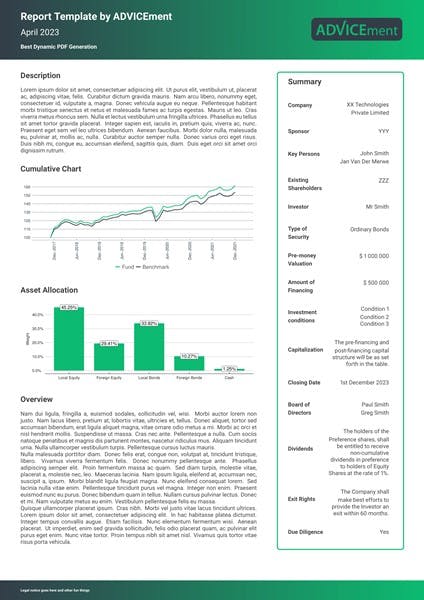
In this section, we provide both an image of the PDF and a part of the corresponding JSON body of the API call used to generate a report. As shown below, this PDF contains dynamic charts, which are discussed in this section.

{
  "documentSettings": {
    "font": "roboto",
    "fontSize": 8,
    "primaryHEXColour": "343D49",
    "secondaryHEXColour": "0dbb72",
    "textHEXColour": "444444",
    "documentName": "Report Template from ADVICEment",
    "topMargin": "-0.1cm",
    "rightMargin": "1cm",
    "bottomMargin": "-0.1cm",
    "leftMargin": "1cm",
    "headheight": "3.13cm",
    "headsep": "0.5cm",
    "footskip": "1.5cm",
    "includehead": true,
    "includefoot": true,
    "showframe": false,
    "header": {
      "headerLine": false,
      "leftContent": "\\begin{tikzpicture} \\node (rectange) [rectangle, shading = axis, shading angle=135, left color=Primary, right color=Secondary, anchor=south west, inner sep=0,outer sep =0, fill = Primary, minimum width = 21cm,  minimum height = 3.0cm] at ([xshift=0.0cm, yshift=0cm]current page.north west)  {}; \\node[right] at ([xshift=0.90cm, yshift=-0.9cm]rectange.north west) {\\bfseries\\color{white}\\huge{Report Template by ADVICEment}}; \\node[right] at ([xshift=0.90cm, yshift=-1.675cm]rectange.north west) {\\color{white}\\LARGE April 2023}; \\node (subtitle) [minimum width=11cm, anchor=north west, text width=11cm, inner sep=0.0cm, outer sep=0] at ([xshift=1.00cm, yshift=-2.25cm]rectange.north west) {\\color{white}\\normalsize\\bfseries{Best Dynamic PDF Generation} }; \\node (logo) [left] at ([xshift=-0.99cm, yshift=-1.5cm]rectange.north east) {\\advGetImage{key = logo, typeKey=logoType, widthKey = logoWidth}}; \\end{tikzpicture}",
      "centerContent": "",
      "rightContent": "",
      "adjustMargin": "1cm"
    },
    "footer": {
      "footerLine": false,
      "leftContent": "\\begin{tikzpicture} \\node (rectange) [rectangle, shading = axis, shading angle=135, left color=Primary, right color=Secondary, anchor=south west, inner sep=0,outer sep =0, fill = Primary, minimum width = 21cm,  minimum height = 1.0cm] at ([xshift=0.0cm, yshift=0cm]current page.south west)  {}; \\node[right] at ([xshift=0.90cm, yshift=0.5cm]rectange.south west) {\\bfseries\\color{white}\\tiny{Legal notice goes here and other fun things}}; \\end{tikzpicture}",
      "centerContent": "",
      "rightContent": "",
      "adjustMargin": "1cm"
    },
    "latexPreamble": " \\usepackage{lipsum} \\usepackage{paracol}"
  },
  "documentContent": {
    "content": [
      {
        "type": "latex",
        "content": "\\sloppy",
        "order": 1
      },
      {
        "type": "latex",
        "content": "\\columnratio{0.65,0.35} \\begin{paracol}{2} \\begin{leftcolumn}",
        "order": 2
      },
      {
        "type": "section",
        "content": "Description",
        "order": 3
      },
      {
        "type": "paragraph",
        "content": "\\lipsum[1]",
        "order": 4
      },
      {
        "type": "section",
        "content": "Cumulative Chart",
        "order": 5
      },
      {
        "type": "chart",
        "content": "ggplot(data=params$performanceGraph)+geom_line(aes(x=as.Date(Date), y=CumulativeBenchmarkReturn, color =' Benchmark ' ), linetype='solid', size=1)+geom_line(aes(x=as.Date(Date), y=CumulativeFundReturn, color =' Fund '), linetype='solid', size=1)+scale_colour_manual(breaks = c(' Fund ',' Benchmark '), values=c('#343D49','#0dbb72')) +theme_economist()+theme(panel.background = element_rect(fill = '#FFFFFF', colour = '#FFFFFF'),plot.background = element_rect(fill = '#FFFFFF', colour = '#FFFFFF'),axis.title.x=element_blank()) +theme(panel.grid.major = element_line(colour = '#A7A8AA', size=0.5))+theme(panel.grid.minor = element_blank())+theme(axis.line = element_line(colour = '#A7A8AA', size = 0.5)) +theme(axis.text = element_text(size = 12, colour = '#28334A'))+theme(axis.text.x = element_text(angle = 90, vjust = 0.5)) +theme(axis.ticks.x = element_line(colour = '#A7A8AA', size = 0.5))+theme(legend.position='bottom', legend.title=element_blank(),legend.background=element_rect(fill = '#FFFFFF', colour = '#FFFFFF'))+ theme(legend.text=element_text(size=16,color='#58595b'))+theme(legend.key = element_rect(fill = 'white'))+theme(axis.title.y=element_text(colour = '#28334A',size=12,margin=unit(c(0,0.2,0,0.2),units='cm'))) +theme(axis.title.y = element_blank()) +theme(legend.spacing=unit(0.1, units = 'cm'),legend.margin=margin(t = 0.1, unit='cm')) +scale_x_date(breaks = seq(as.Date('2004-06-30'), as.Date('2050-06-30'), by='6 months'), labels=date_format('%b-%Y'), expand = c(0.1, 0.1))+scale_y_continuous(breaks = pretty(c(params$performanceGraph$CumulativeFundReturn,params$performanceGraph$CumulativeBenchmarkReturn),n=8),labels=dollar_format(prefix='',big.mark = ' '))",
        "order": 5,
        "height": 4,
        "width": 10
      }
....
  "performanceGraph":   [
      {
        "Date":  "2017-11-30",
        "Benchmark":  -0.97267,
        "Fund":  -0.63828,
        "CumulativeFundReturn":  100,
        "CumulativeBenchmarkReturn":  100
      },
      {
        "Date":  "2017-12-31",
        "Benchmark":  5.65561,
        "Fund":  5.48700,
        "CumulativeFundReturn":  111.874435153,
        "CumulativeBenchmarkReturn":  109.896525389
      },
      {
        "Date":  "2018-01-31",
        "Benchmark":  1.85912,
        "Fund":  1.93257,
        "CumulativeFundReturn":  114.036486924,
        "CumulativeBenchmarkReturn":  111.939633672
      },
      {
        "Date":  "2018-02-28",
        "Benchmark":  3.93107,
        "Fund":  4.04714,
        "CumulativeFundReturn":  118.651703201,
        "CumulativeBenchmarkReturn":  116.340059029
      }
....
There are two charts being created in the PDF document. These charts are generated using the R package ggplot2, and their code is provided within the JSON. The charts are part of the document content and are represented as objects with the "type": "chart" key-value pair.
Cumulative Chart
{
  "type": "chart",
  "content": "ggplot(data=params$performanceGraph)+geom_line(aes(x=as.Date(Date), y=CumulativeBenchmarkReturn, color =' Benchmark ' ), linetype='solid', size=1)+geom_line(aes(x=as.Date(Date), y=CumulativeFundReturn, color =' Fund '), linetype='solid', size=1)+scale_colour_manual(breaks = c(' Fund ',' Benchmark '), values=c('#343D49','#0dbb72')) +theme_economist()+theme(panel.background = element_rect(fill = '#FFFFFF', colour = '#FFFFFF'),plot.background = element_rect(fill = '#FFFFFF', colour = '#FFFFFF'),axis.title.x=element_blank()) +theme(panel.grid.major = element_line(colour = '#A7A8AA', size=0.5))+theme(panel.grid.minor = element_blank())+theme(axis.line = element_line(colour = '#A7A8AA', size = 0.5)) +theme(axis.text = element_text(size = 12, colour = '#28334A'))+theme(axis.text.x = element_text(angle = 90, vjust = 0.5)) +theme(axis.ticks.x = element_line(colour = '#A7A8AA', size = 0.5))+theme(legend.position='bottom', legend.title=element_blank(),legend.background=element_rect(fill = '#FFFFFF', colour = '#FFFFFF'))+ theme(legend.text=element_text(size=16,color='#58595b'))+theme(legend.key = element_rect(fill = 'white'))+theme(axis.title.y=element_text(colour = '#28334A',size=12,margin=unit(c(0,0.2,0,0.2),units='cm'))) +theme(axis.title.y = element_blank()) +theme(legend.spacing=unit(0.1, units = 'cm'),legend.margin=margin(t = 0.1, unit='cm')) +scale_x_date(breaks = seq(as.Date('2004-06-30'), as.Date('2050-06-30'), by='6 months'), labels=date_format('%b-%Y'), expand = c(0.1, 0.1))+scale_y_continuous(breaks = pretty(c(params$performanceGraph$CumulativeFundReturn,params$performanceGraph$CumulativeBenchmarkReturn),n=8),labels=dollar_format(prefix='',big.mark = ' '))",
  "order": 5,
  "height": 4,
  "width": 10
}
This chart is a line chart showing the Cumulative Benchmark Return and the Cumulative Fund Return. The code for this chart is provided in the "content" field as a ggplot2 expression. The chart's dimensions are set with the "height" and "width" fields, measuring 4 units high and 10 units wide.
Asset Allocation Chart
{
  "type": "chart",
  "content": "ggplot(params$assetAllocationChart,aes(x = factor(Name, levels = params$assetAllocationChart$Name), y = Weight))+geom_bar(stat='identity', position=position_dodge(width=1), width = 0.75, fill = '#0dbb72')+geom_label(aes(label = Label), fill = 'white', colour = 'black', position= position_dodge(width=1), size = 5) +theme_economist()+scale_colour_economist()+theme(legend.position='bottom')+theme(legend.position='bottom', legend.direction = 'horizontal', legend.title=element_blank(),legend.background=element_rect(fill = '#FFFFFF', colour = '#FFFFFF'),legend.box.background=element_rect(fill = '#FFFFFF', colour = '#FFFFFF'),legend.key=element_rect(fill = '#FFFFFF', colour = '#FFFFFF'))+theme(legend.text=element_text(size=12,color='#2D2323',face='plain'))+guides(fill = guide_legend(nrow = 1))+theme(panel.background = element_rect(fill = '#FFFFFF', colour = '#FFFFFF'),plot.background = element_rect(fill = '#FFFFFF', colour = '#FFFFFF')) +theme(panel.grid.major = element_line(colour = 'lightgrey', size=0.5))+theme(panel.grid.minor = element_blank())+theme(axis.title.x=element_blank()) +theme(axis.title.y=element_text(colour = '#2D2323',size=12,margin=unit(c(0.0,0.25,0.0,0.25),units='cm'))) +theme(legend.spacing.x = unit(0.1, 'cm'))+theme(axis.text = element_text(size=12,color='#2D2323', face='plain'))+theme(axis.title = element_text(size=12,color='#2D2323', face='plain'))+scale_y_continuous(breaks = pretty(c(params$assetAllocationChart$Weight),n=6),labels=percent_format(accuracy = 0.1))+labs(y='Weight')+coord_cartesian(clip = 'off')",
  "order": 7,
  "height": 3.5,
  "width": 10
}
This chart is a bar chart displaying the weight of each asset in the portfolio. The ggplot2 code for generating this chart is provided in the "content" field. The chart's dimensions are set with the "height" and "width" fields, measuring 3.5 units high and 10 units wide.
Once the R code for generating these charts is executed, the resulting chart images are incorporated into the PDF document as specified by their respective order in the "documentContent" section of the JSON data.
For more information on how to use ggplot2 and create charts consult the ggplot2 official page or the ggplot2 cheat graphic.
Data and Layout Separation
In the aforementioned examples, it is crucial to recognize that the table and chart data reside independently from the PDF layout within the JSON. This distinction is significant as it allows for seamless updates to the document's underlying data in the JSON, automatically reflecting the changes within the document. This approach offers considerable benefits for developers tasked with PDF generation, streamlining their workflow and enhancing efficiency.
General JSON to PDF Postman Collection
To make it easier to test the General JSON to PDF Endpoint, we've provided a ready-to-use Postman collection. This allows you to generate the PDFs mentioned above with ease. Feel free to use the link below to access the collection and explore its features, or even fork the collection to customize it according to your needs.
Harnessing LaTeX and JSON for Effortless Customization
In conclusion, this article has demonstrated the versatility and efficiency of using JSON in conjunction with LaTeX to generate PDF documents through API calls. By showcasing three distinct examples, we have illustrated the ease of adapting the layout and content of PDFs by simply modifying the JSON payload. LaTeX, while possessing a steep learning curve, offers unparalleled control over the appearance and structure of documents. The General JSON to PDF Template introduced in this article streamlines the PDF generation process by allowing developers to make layout and content changes within the JSON body of the API call, eliminating the need to modify templates. This innovative approach saves time, reduces complexity, and enhances the developer experience in creating professional and aesthetically pleasing PDF documents.

